Introduction:
In this post, I am sharing a project I completed as part of my machine learning course at Ashoka University. The objective was to leverage machine learning to understand the extent of urbanisation in the city of Delhi. Using the concept of built-up areas as a proxy for urban areas, I applied Random Forest machine learning algorithm to estimate the built-up area in Delhi.
Methodology:
Obtaining Delhi Boundary Geometry:
To initiate the project, I obtained the precise boundary geometry of Delhi using the FAO/GAUL/2015/level2 dataset. This enabled me to focus specifically on the area of interest and streamline the analysis.
var delhi = ee.FeatureCollection("FAO/GAUL/2015/level2").filter(ee.Filter.eq('ADM2_NAME','Delhi')).geometry();
Filtering Sentinel-2 Imagery:
Next, I accessed the Sentinel-2 satellite imagery from the COPERNICUS/S2_SR image collection. To ensure high-quality data, I filtered the imagery based on a cloud cover percentage of less than 30% and a date range of January 1, 2019, to December 31, 2019. Additionally, I restricted the imagery to be within the bounds of Delhi, using the previously acquired boundary geometry. Subsequently, I selected the relevant spectral bands (B4, B3, B2) for the analysis.
// Code snippet 1: Filtering Sentinel-2 imagery
var sentinel2 = ee.ImageCollection("COPERNICUS/S2_SR")
  .filterBounds(delhi)
  .filterDate("2019-01-01", "2019-12-31")
  .filter(ee.Filter.lt("CLOUDY_PIXEL_PERCENTAGE", 30))
  .select(["B4", "B3", "B2"]);
Creating the Composite Image:
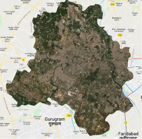
Afterwards, I created a composite image by taking the median of the filtered images and clipped it to the boundary of Delhi. The resulting composite image provided a comprehensive representation of the land cover in the region.
I then created a composite image by taking the median of the filtered images and clipped it to the boundary of Delhi. This composite image provided a comprehensive representation of the land cover in the region.
// Code snippet 2: Creating the composite image
var composite = sentinel2.median().clip(delhi);
Visualising the Composite Image
To visualise the composite image, I applied a colour visualisation scheme using the red, green, and blue bands. This enhanced the image and provided valuable insights into the distribution of different land cover types within Delhi.
// Code Snippet: Visualising the Composite Image

// Apply colour visualization parameters
var visualizationParams = {
  bands: ['B4', 'B3', 'B2'],
  min: 0.0,
  max: 3000
};

// Display the composite image

Map.addLayer(compositeImage, visualizationParams, 'Composite Image');
Composite Image
Land Cover Classification Training Data:
I manually annotated approximately 500 urban and non-urban points across Delhi to create the training data. I uploaded them to GEE assets as feature collection. I utilised that feature collection consisting of urban and non-urban points. Merging these collections provided a comprehensive set of training data for the classification process.
// Code Snippet: Utilising the Feature Collection for Classification
// Load the feature collections of urban and non-urban points
var urbanPoints = ee.FeatureCollection("projects/ee-najah/assets/urban_points");
var nonUrbanPoints = ee.FeatureCollection("projects/ee-najah/assets/non_urban_points");

// Merge the urban and non-urban points collections
var trainingData = urbanPoints.merge(nonUrbanPoints);
Overlaying Training Points and Extracting Training Data:
Next, I overlayed the training points on the composite image to extract the necessary training data. This involved sampling regions within a specified scale of 10 units using the “sampleRegions” function, which resulted in the training data consisting of land cover labels associated with each region.
// Code Snippet: Overlaying Training Points on the Composite Image
// Sample regions within a specified scale of 10 units
var trainingData = compositeImage.sampleRegions({
  collection: trainingData,
  scale: 10,
  properties: ['land_cover'],
});
Splitting the Dataset:
To evaluate the accuracy of the classification model, I split the dataset into training and testing sets. The training set was used to train the machine learning model, while the testing set was utilized to assess the model’s performance.
// Code snippet 5: Splitting the dataset into training and testing sets
var split = 0.8; // 80% for training, 20% for testing

var trainingData = trainingData.randomColumn('split')
var training = trainingData.filter(ee.Filter.lt('split', split));
var testing = trainingData.filter(ee.Filter.gte('split', split));
Training the Random Forest Classifier:
Using the training data, I trained a random forest classifier with the “smileRandomForest” algorithm provided by Earth Engine. The classifier was trained with 50 trees, and the land cover property was used as the target class. The input properties for classification were derived from the band names of the composite image.
// Code Snippet: Training the Random Forest Classifier

// Train a random forest classifier with 500 trees
var classifier = ee.Classifier.smileRandomForest(500)
  .train({
    features: training,
    classProperty: 'land_cover',
    inputProperties: ['B4', 'B3', 'B2']
  });
Applying the Classifier to Generate Land Cover Classification Map
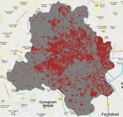
Finally, I applied the trained classifier to the composite image to generate a land cover classification map. The classified image assigned distinct colours to different land cover classes, with the colour palette including shades of grey, brown, blue, and green. This visualisation provided a clear understanding of the land cover distribution in Delhi during the year 2019.
// Code Snippet: Applying the Classifier to Generate Land Cover Classification Map

// Apply the trained classifier to the composite image
var classified = compositeImage.classify(classifier);

// Display the land cover classification map
Map.addLayer(classified, { palette: ['gray', 'red'] }, 'Land Cover Classification');
Land Classification Map
Accuracy Assessment:
To assess the accuracy of the classification model, I calculated the confusion matrix using the testing dataset. The confusion matrix provided insights into the model’s performance, including metrics such as overall accuracy, producer’s accuracy, and user’s accuracy.
// Code snippet 7: Calculating the confusion matrix for accuracy assessment
var testAccuracy = testing
    .classify(classifier)
    .errorMatrix('class', 'classification');

print('Confusion Matrix:', testAccuracy);
print('Overall Accuracy:', testAccuracy.accuracy());
Calculating Urban Area Percentage:
To understand the extent of urbanization, we calculated the area covered by the urban class within Delhi. We also calculated the total area of Delhi to determine the percentage of urban area.
// New Code Snippet: Calculating urban area percentage

// Calculating area of urban class
var urban = classified.select('classification').eq(1);

// Calculate the pixel area in square kilometer for urban
var area_urban = urban.multiply(ee.Image.pixelArea()).divide(1000 * 1000);

// Reducing the statistics for urban area in Delhi
var stat_urban = area_urban.reduceRegion({
  reducer: ee.Reducer.sum(),
  geometry: delhi,
  scale: 100,
  maxPixels: 1e10
});

// Get the sum of pixel values representing urban area
var area_urban_sum = ee.Number(stat_urban.get('classification'));

// Calculate the pixel area in square kilometer for Delhi
var area_delhi = ee.Image.pixelArea().clip(delhi).divide(1000 * 1000);

// Reducing the statistics for Delhi
var stat_delhi = area_delhi.reduceRegion({
  reducer: ee.Reducer.sum(),
  geometry: delhi,
  scale: 100,
  maxPixels: 1e10
});

// Get the sum of pixel values representing Delhi area
var area_delhi_sum = ee.Number(stat_delhi.get('area'));

// Calculate the percentage of urban area
var percentage_urban_area = area_urban_sum.divide(area_delhi_sum).multiply(100);

// Print the urban area in square kilometers
print('Urban Area (in sq.km):', area_urban_sum);

// Print the total area of Delhi
print('Delhi Area (in sq.km):', area_delhi_sum);

// Print the percentage of urban area
print('Percentage of urban area:', percentage_urban_area);
Exporting the Results:
Lastly, I exported the classified image and the confusion matrix results to Google Drive for further analysis and sharing with collaborators.
// Code snippet 8: Exporting the classified image and confusion matrix to Google Drive
Export.image.toDrive({
  image: classified,
  description: 'classified_image',
  folder: 'GEE_Classification_Results',
  scale: 10,
  region: delhi
});

Export.table.toDrive({
  collection: testAccuracy,
  description: 'confusion_matrix',
  folder: 'GEE_Classification_Results',
  fileFormat: 'CSV'
});
Results and Conclusion
The land cover classification analysis using the basic Random Forest model achieved an overall accuracy of 87%, indicating the model’s effectiveness in accurately classifying land cover types in Delhi based on satellite imagery data.
To further improve the classification results, additional enhancements can be implemented, such as incorporating spectral indices like NDVI (Normalised Difference Vegetation Index) or NDBI (Normalised Difference Built-up Index) to provide additional information for distinguishing different land cover types.
Hyperparameter optimisation can be performed to fine-tune the Random Forest model, adjusting parameters such as the number of trees, tree depth, and feature subsampling, with the potential to achieve higher accuracy.
This project primarily focused on land cover classification in Delhi, but there is potential for extending the analysis to other Indian cities. Analysing the model’s performance in different urban environments would provide valuable insights into its generalisability and scalability.
The classification results suggest that approximately 78% of Delhi can be classified as urban, highlighting the significant urbanisation within the city.
By tracking the historical growth of urban areas in Delhi using satellite imagery, it is possible to gain a deeper understanding of urban expansion patterns over time.